
Valve sizing
Technical whitepaper
Scope
Valve size often is described by the nominal size of the end connections, but a more important measure is the flow that the valve can provide. And determining flow through a valve can be simple.
This technical bulletin shows how flow can be estimated well enough to select a valve size—easily, and without complicated calculations. Included are the principles of flow calculations, some basic formulas, and the effects of specific gravity and temperature. Also given are six simple graphs for estimating the flow of water or air through valves and other components and examples of how to use them.
Sizing valves
The graphs cover most ordinary industrial applications—from the smallest metering valves to large ball valves, at system pressures up to 10 000 psig and 1000 bar.
The water formulas and graphs apply to ordinary liquids—and not to liquids that are boiling or flashing into vapours, to slurries (mixtures of solids and liquids), or to very viscous liquids.
The air formulas and graphs apply to gases that closely follow the ideal gas laws, in which pressure, temperature, and volume are proportional. They do not apply to gases or vapours that are near the pressure and temperature at which they liquefy, such as a cryogenic nitrogen or oxygen.
For convenience, the air flow graphs show gauge pressures, whereas the formulas use absolute pressure (gauge pressure plus one atmosphere). All the graphs are based on formulas adapted from ISA S75.01, Flow Equations for Sizing Control Valves.1
Safe product selection
When selecting a product, the total system design must be considered to ensure safe, trouble-free performance. Function, material compatibility, adequate ratings, proper installation, operation, and maintenance are the responsibilities of the system designer and user.
Flow calculation principles
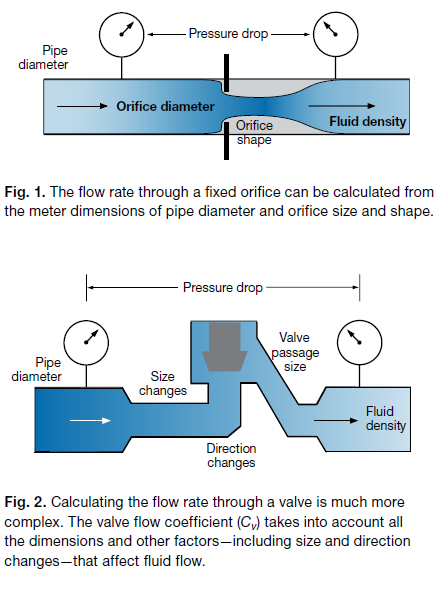
The principles of flow calculations are illustrated by the common orifice flow meter (Fig. 1). We need to know only the size and shape of the orifice, the diameter of the pipe, and the fluid density. With that information, we can calculate the flow rate for any value of pressure drop across the orifice (the difference between inlet and outlet pressures).
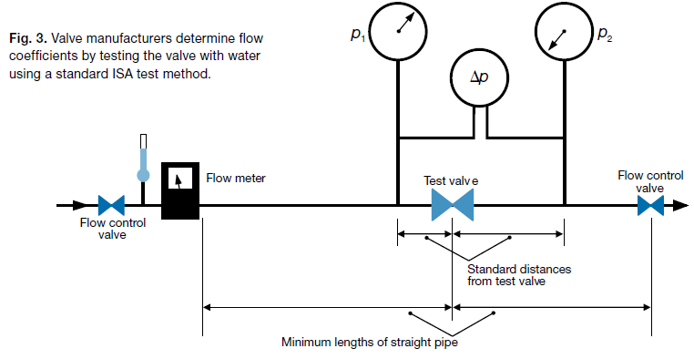
For a valve, we also need to know the pressure drop and the fluid density. But in addition to the dimensions of pipe diameter and orifice size, we need to know all the valve passage dimensions and all the changes in size and direction of flow through the valve.
However, rather than doing complex calculations, we use the valve flow coefficient, which combines the effects of all the flow restrictions in the valve into a single number (Fig. 2).
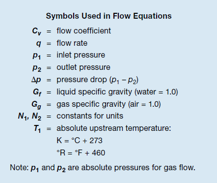
Valve manufacturers determine the valve flow coefficient by testing the valve with water at several flow rates, using a standard test method2 developed by the Instrument Society of America for control valves and now used widely for all valves.
Flow tests are done in a straight piping system of the same size as the valve, so that the effects of fittings and piping size changes are not included (Fig. 3).
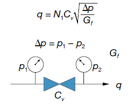
Liquid flow
Because liquids are in-compressible fluids, their flow rate depends only on the difference between the inlet and outlet pressures (Dp, pressure drop). The flow is the same whether the system pressure is low or high, so long as the difference between the inlet and outlet pressures is the same. This equation shows the relationship:
The water flow graphs (pages 6 and 7) show water flow as a function of pressure drop for a range of Cv values.
Gas flow
Gas flow calculations are slightly more complex, because gases are compressible fluids whose density changes with pressure. In addition, there are two conditions that must be considered—low pressure drop flow and high pressure drop flow.
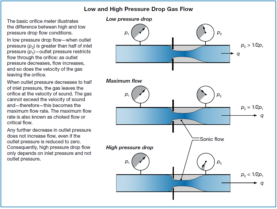
This equation applies when there is low pressure drop flow—outlet pressure (p2) is greater than one half of inlet pressure (p1):
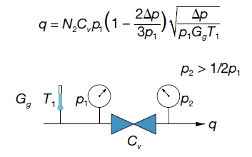
The low pressure drop air flow graphs (pages 8 and 9) show low pressure drop air flow for a valve with a Cv of 1.0, given as a function of inlet pressure (p1) for a range of pressure drop (Δp) values.
When outlet pressure (p2) is less than half of inlet pressure (p1)—high pressure drop—any further decrease in outlet pressure does not increase the flow because the gas has reached sonic velocity at the orifice, and it cannot break that “sound barrier.”
The equation for high pressure drop flow is simpler because it depends only on inlet pressure and temperature, valve flow coefficient, and specific gravity of the gas:
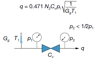
The high pressure drop air flow graphs show high pressure drop air flow as a function of inlet pressure for a range of flow coefficients.
Effects of specific gravity
The flow equations include the variables Gf and Gg—liquid specific gravity and gas specific gravity—which are the density of the fluid compared to the density of water (for liquids) or air (for gases).
However, specific gravity is not accounted for in the graphs, so a correction factor must be applied, which includes the square root of G. Taking the square root reduces the effect and brings the value much closer to that of water or air, 1.0.
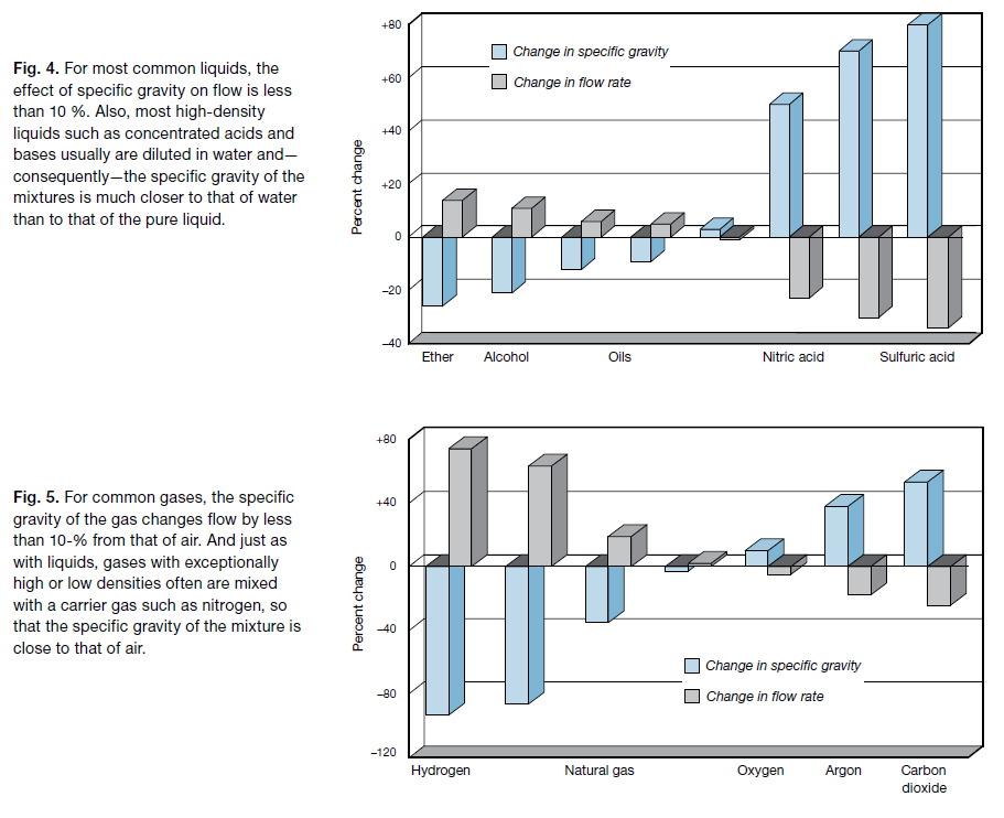
For example, the specific gravity of sulfuric acid is 80 % higher than that of water, yet it changes flow by just 34 %. The specific gravity of ether is 26 % lower than that of water, yet it changes flow by only 14 %.
Figure 4 shows how the significance of specific gravity on liquid flow is diminished by taking its square root. Only if the specific gravity of the liquid is very low or very high will the flow change by more than 10 % from that of water.
The effect of specific gravity on gases is similar. For example, the specific gravity of hydrogen is 93 % lower than that of air, but it changes flow by just 74 %. Carbon dioxide has a specific gravity 53 % higher than that of air, yet it changes flow by only 24 %. Only gases with very low or very high specific gravity change the flow by more than 10 % from that of air.
Figure 5 shows how the effect of specific gravity on gas flow is reduced by use of the square root.
Effects of temperature
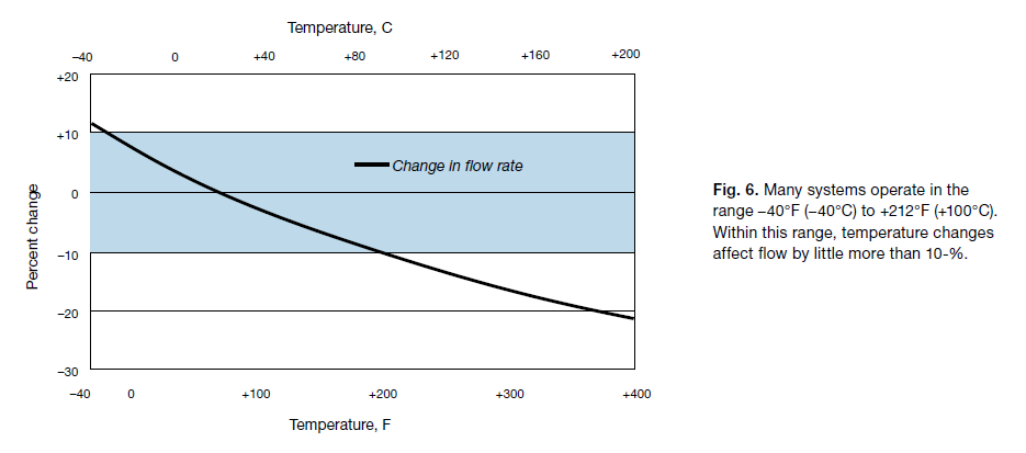
Temperature usually is ignored in liquid flow calculations because its effect is too small. Temperature has a greater effect on gas flow calculations, because gas volume expands with higher temperature and contracts with lower temperature. But—similar to specific gravity—temperature affects flow by only a square-root factor. For systems that operate between –40°F (–40°C) and +212°F (+100°C), the correction factor is only +12 to –11 %.
Figure 6 shows the effect of temperature on volumetric flow over a broad range of temperatures. The plus-or-minus 10 % range covers the usual operating temperatures of most common applications.
Other services
As noted above, this technical bulletin covers valve sizing for many common applications and services. What about viscous liquids, slurries, or boiling and flashing liquids? Suppose vapors, steam, and liquefied gases are used? How are valves sized for these other services?
Such applications are beyond the scope of this document, but the ISA standards S75.01 and S75.02 contain a complete set of formulas for sizing valves that will be used in a variety of special services, along with a description of flow capacity test principles and procedures. These and other ISA publications are listed in the references. Also, most standard engineering handbooks have sections on fluid mechanics. Several of these are given in the references, as well.
Cited references
1. ISA S75.01, Flow Equations for Sizing Control Valves, Standards and Recommended Practices for Instrumentation and Control, 10th ed., Vol. 2, 1989.
2. ISA S75.02, Control Valve Capacity Test Procedure, Standards and Recommended Practices for Instrumentation and Control, 10th ed., Vol. 2, 1989.
Other references
L. Driskell, Control-Valve Selection and Sizing, ISA, 1983.
J.W. Hutchinson, ISA Handbook of Control Valves, 2nd ed., ISA, 1976.
Chemical Engineers’ Handbook, 4th ed., Robert H. Perry, Cecil H. Chilton, and Sidney D. Kirkpatrick, Ed., McGraw-Hill, New York.
Instrument Engineers’ Handbook, revised ed., Béla G. Lipták and Kriszta Venczel, Ed., Chilton, Radnor, PA.
Piping Handbook, 5th ed., Reno C. King, Ed., McGraw-Hill, New York.
Standard Handbook for Mechanical Engineers, 7th ed., Theodore Baumeister and Lionel S. Marks, Ed., McGraw-Hill, New York
** This Technical Whitepaper was written by and for Swagelok Corporation.
Safe Product Selection
When selecting a product, the total system design must be considered to ensure safe, trouble-free performance. Function, material compatibility, adequate ratings, proper installation, operation, and maintenance are the responsibilities of the system designer and user.
Swagelok - TM Swagelok Company
© 1994, 1995, 2000, 2002 Swagelok Company
December 2007, R4
MS-06-84-E
